Techno-economic optimization of hybrid renewable systems for sustainable energy solutions

Figure 3: Flowchart for the techno-economic optimization process of the hybrid renewable energy system outlines a comprehensive sequence of steps for optimizing hybrid renewable energy systems, integrating wind, solar, and geothermal resources. The process begins with Data Collection, which is crucial for gathering all necessary data that influences system design. The collected data spans environmental conditions, resource availability, demand forecasts, and economic parameters, all of which form the basis for subsequent decisions. Without accurate and comprehensive data, the optimization process cannot proceed effectively, as the system’s performance and financial feasibility directly depend on this information. Environmental data, such as wind speed and solar irradiance, inform energy production estimates, while economic data ensures the optimization aligns with financial goals, helping identify the most cost-effective solution. Moreover, understanding demand patterns ensures the designed system can meet load requirements effectively, without excess production or deficiencies in energy supply. The first step, Data Collection, involves gathering environmental, resource, demand, and economic data to inform the system design. This data provides the foundation for accurately modeling energy production, system performance, and financial viability. In this step, wind speed, solar irradiance, geothermal heat flow, demand forecasts, and economic parameters like fuel costs and capital costs are collected. Accurate data on wind speed and solar radiation ensures that energy production models reflect real-world conditions, while demand forecasts inform the design of the energy system to meet varying loads. Without comprehensive data, optimization and financial assessments cannot be accurately conducted.

For wind energy, the equation 

. is used, where \({E_{wind}}\) is the energy generated from wind (kWh), \(\rho\) represents the air density (kg/m³), A is the area swept by the turbine blades (m²), \({C_p}\) is the power coefficient of the turbine (dimensionless), and V is the wind velocity (m/s). This equation calculates the energy generation from wind, which is influenced by factors such as air density, wind speed, and turbine efficiency. For solar energy, the Eq. 

is employed, where \({E_{solar}}\) is the energy generated from solar (kWh), \({A_{panel}}\) is the area of the solar panel (m²), G is the solar irradiance (W/m²), \({\eta _{panel}}\) represents the efficiency of the solar panel (dimensionless), \({\beta _{solar}}\) is the temperature coefficient of the solar panel (per °C), T is the temperature (°C), and \({T_{ref}}\) is the reference temperature (°C). This equation accounts for the effects of temperature on solar panel efficiency, as temperature increases can reduce the panel’s ability to generate energy. Geothermal energy generation is modeled using the Eq. 

where \({E_{geo}}\) is the energy generated from geothermal sources (kWh), \(\dot {Q}\) is the geothermal heat flow (W), \(\Delta T\) is the temperature difference (°C), and \({C_p}\) is the specific heat capacity of the geothermal fluid (J/kg°C). This equation estimates the energy produced based on the heat transfer and temperature variation in geothermal systems.

After Data Collection, the next step is Define System Objectives, where optimization goals like cost reduction and energy efficiency are set. These objectives help guide the optimization process by focusing on the most important outcomes such as minimizing costs while maximizing energy production. Defining clear system objectives ensures that the project remains focused on achieving the best possible performance while meeting financial and environmental goals. The main objectives in this phase typically include reducing capital and operational costs, increasing system efficiency, and maximizing renewable energy use. Setting these goals ensures that every step in the optimization process is aligned with achieving the desired results.

Setting optimization goals involves ensuring that energy production, cost efficiency, and sustainability are the key performance indicators. These goals drive the system design process and ultimately determine the techno-economic viability of the project. By focusing on reducing costs while maximizing energy efficiency, the system can provide a reliable power supply without exceeding budget constraints. Defining system objectives helps prioritize the design considerations, ensuring that the system is both technically viable and economically sustainable. Without these clear objectives, the system design may lack direction and fail to meet necessary performance or financial targets. The capital (CAPEX) and operational (OPEX) expenditures used in this study are derived from literature values reported in references^6,7. These values were adapted to reflect the local context by incorporating regional cost adjustments, inflation indexing, and technology-specific parameters relevant to the system design. All values were normalized in alignment with the economic modeling framework presented in the total system cost is determined by the Eq. 

where \({C_{total}}\) is the total system cost (in dollars), \({C_{wind}}\) represents the cost of wind turbines (in dollars), \({C_{solar}}\) is the cost of solar panels (in dollars), \({C_{geo}}\) refers to the cost of geothermal systems (in dollars), \({C_{storage}}\) is the cost of energy storage systems (in dollars), and \({C_{control}}\) indicates the cost of control systems (in dollars). This equation calculates the overall investment required to deploy and operate the hybrid renewable system by aggregating the individual costs of each component. The energy efficiency objective is represented by the equation 

where \({\eta _{total}}\) is the total system efficiency (in percentage), \({E_{total}}\) refers to the total energy output (in kWh), and \({E_{available}}\) represents the total available energy from all sources (in kWh). This equation helps evaluate how effectively the hybrid system utilizes the available energy resources to generate power, where a higher efficiency percentage indicates better utilization of the renewable resources.

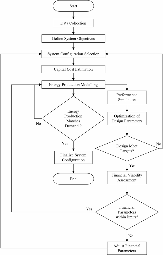
Flow chart for the techno-economic optimization process of the hybrid renewable energy system.

In terms of sustainability, the objective is represented by the equation 

where \(GH{G_{total}}\) represents the total greenhouse gas emissions (in kg CO₂), \(GH{G_{wind}}\) refers to emissions associated with wind (in kg CO₂), \(GH{G_{solar}}\) represents emissions associated with solar (in kg CO₂), \(GH{G_{geo}}\) represents emissions associated with geothermal (in kg CO₂), and \(GH{G_{offset}}\) is the offset from carbon credits (in kg CO₂). This equation calculates the environmental impact of the hybrid energy system, ensuring that greenhouse gas emissions are minimized through the adoption of renewable energy sources and the use of carbon offset mechanisms. Once the System Objectives are defined, the next step is System Configuration Selection, where the most suitable combination of renewable energy sources is chosen based on available resources. The choice of energy sources depends on the specific environmental conditions at the installation site, such as wind speed, solar irradiance, and geothermal heat flow. The objective is to select a mix of renewable resources that can efficiently meet the energy demand while being cost-effective. Each resource—wind, solar, and geothermal—has unique characteristics that must be optimized based on their availability. This step ensures that the hybrid system is appropriately designed to take advantage of the most effective renewable resources for the location. In the next step, the optimal combination of renewable energy sources is chosen to meet the energy demand while considering environmental conditions. The selection of energy sources is driven by factors such as location-specific wind speed, solar irradiance, and geothermal heat flow, with each energy source contributing to the system’s overall efficiency. The goal is to choose a mix of wind, solar, and geothermal systems that will work together to provide consistent and reliable power. The energy generation potential from each source must be balanced to minimize costs and maximize efficiency. By evaluating the energy mix, system designers ensure that the chosen configuration is sustainable, cost-effective, and capable of meeting load requirements.

The total energy production from the hybrid system is calculated using the equation 

where \({E_{hybrid}}\) represents the total energy generated by the hybrid system (in kWh), \({E_{wind}}\) is the energy generated from wind (in kWh), \({E_{solar}}\) is the energy produced from solar (in kWh), and \({E_{geo}}\) denotes the energy produced from geothermal sources (in kWh). This equation sums the individual energy contributions from each renewable source to determine the total energy output of the hybrid system. The renewable resource availability factor is represented by the Eq. 

where \({F_{availability}}\) indicates the renewable resource availability factor (in percentage), \({E_{available}}\) is the available energy from resources (in kWh), and \({E_{max}}\) represents the maximum possible energy generation (in kWh). This factor helps assess how effectively the hybrid system utilizes the available resources in relation to their maximum potential, ensuring that the system is designed to optimize resource availability. The system cost efficiency is calculated by the Eq. 

where \({\eta _{cost}}\) is the cost efficiency of the system (in percentage), \({C_{total}}\) is the total capital cost of the system (in dollars), and \({E_{hybrid}}\) is the total energy generated by the system (in kWh). This equation evaluates how cost-effective the hybrid energy system is by comparing the capital investment against the total energy production, with a lower cost efficiency value indicating that the system is less economical in terms of energy production per unit cost. Following System Configuration Selection, the next step is Capital Cost Estimation, where the initial investment required for the system components is calculated. This estimation includes all costs related to the procurement and installation of wind turbines, solar panels, geothermal systems, storage units, and control systems. Estimating the capital cost is essential for determining the overall feasibility of the project, as it provides the baseline for the financial evaluation. Accurate capital cost estimation allows for the identification of potential cost-saving opportunities and informs decision-making regarding system size and components. This step ensures that the project remains within budget while achieving the desired technical performance. Capital cost estimation involves calculating the total investment needed for the system components, considering factors such as the number and size of components, installation costs, and associated infrastructure. This estimation is crucial for assessing the project’s financial feasibility and ensuring that the costs align with the financial objectives. A comprehensive capital cost estimation helps identify areas where cost reductions may be necessary and provides a solid financial basis for the project. It is also essential for determining the return on investment (ROI) and for setting appropriate funding and financing strategies. Accurate cost estimation also provides stakeholders with clear financial expectations and helps prevent budget overruns. The total capital cost of the system is calculated using the Eq. 

where \({C_{total}}\) represents the total capital cost (in dollars), \({C_{wind}}\) is the cost associated with wind turbines (in dollars), \({C_{solar}}\) denotes the cost of solar panels (in dollars), \({C_{geo}}\) represents the cost of geothermal systems (in dollars), \({C_{storage}}\) refers to the cost of energy storage systems (in dollars), and \({C_{control}}\) is the cost for control systems (in dollars). This equation adds up the individual costs of all the components necessary for the system to function, providing a comprehensive picture of the initial investment required for deployment. To assess the cost-efficiency of the system in terms of energy production, the cost per unit of energy is calculated using the equation

where \({C_{unit}}\) is the cost per unit of energy (in dollars per kWh), \({C_{total}}\) is the total capital cost (in dollars), and \({E_{hybrid}}\) is the total energy produced by the system (in kWh). This equation indicates how much the system costs per unit of energy produced, helping to assess whether the energy generation is financially viable and cost-effective. Another essential calculation in the financial assessment is the break-even point for capital recovery, which determines the time required for the system to generate enough revenue to recover the initial investment. This is calculated using the equation 

where \({T_{break – even}}\) represents the time to break even (in years), \({C_{total}}\) is the total capital cost (in dollars), and \({R_{annual}}\) is the annual revenue generated from the system (in dollars). This equation helps estimate how many years it will take for the system to pay back its initial investment based on the annual income it generates. By determining this time frame, stakeholders can evaluate whether the system is a viable long-term investment, ensuring that the return on investment (ROI) is achieved within an acceptable period. Energy production modeling is a crucial step in assessing the expected energy output of the hybrid renewable energy system based on environmental data. This step involves simulating how much energy each renewable resource—wind, solar, and geothermal—can generate under varying environmental conditions, such as changes in weather, time of day, and seasonal variations. Accurate modeling ensures that the system can consistently meet the energy demand, providing both reliability and stability. In this step, the environmental data collected earlier is used to estimate the generation potential from each energy source, factoring in potential downtimes or fluctuations in availability. Additionally, it helps in optimizing the system design by assessing the expected capacity factor and generation patterns, guiding decisions about system component sizing and storage needs.

The total energy generation by the hybrid system is determined by adding the energy produced from all renewable sources, wind, solar, and geothermal. This is captured by the equation 

where \({E_{total}}\) represents the total energy generated by the system (in kWh), \({E_{wind}}\) is the energy produced by wind (in kWh), \({E_{solar}}\) is the energy produced by solar (in kWh), and \({E_{geo}}\) is the energy produced from geothermal sources (in kWh). This equation provides the total amount of electricity generated by the system, ensuring the integrated use of multiple renewable resources to meet energy demand. The energy produced from each source is combined to evaluate the system’s overall performance, helping identify any shortfalls or excess production relative to demand.

Next, the energy capacity factor (CF) is an important metric for evaluating how effectively the system operates relative to its rated capacity. This is calculated by the equation 

where CF represents the capacity factor (in percentage), \({E_{actual}}\) is the actual energy output of the system (in kWh), and \({E_{rated}}\) is the rated capacity of the system (in kWh). The capacity factor measures how much energy is generated relative to the maximum potential energy output. A higher capacity factor indicates a more efficient system, as it consistently operates near its rated capacity. This metric helps identify inefficiencies or overestimations in energy generation potential, enabling further optimization of the system design. Lastly, the energy availability ratio is calculated to assess whether the energy produced by the system meets the demand requirements. The equation 

which determines the energy availability ratio, where \({A_{energy}}\) is the energy availability ratio (in percentage), \({E_{available}}\) is the energy produced by the system (in kWh), and \({E_{demand}}\) is the energy demand or load (in kWh). This equation helps assess the adequacy of the hybrid system’s energy generation to meet the required energy demand. A higher energy availability ratio indicates that the system consistently meets or exceeds demand, while a lower ratio may suggest the need for additional energy production capacity or storage to ensure reliable power supply. Performance simulation involves modeling the system’s behavior under different environmental scenarios to assess its overall efficiency and reliability. This step simulates how the system would perform during real-world conditions such as varying weather patterns, fluctuating renewable resource availability, and changing energy demands. By running these simulations, the team can identify weaknesses or inefficiencies in the system, ensuring that it can operate optimally despite external factors. The simulation also provides insight into the potential impacts of system downtime or resource unavailability, helping to fine-tune system components and optimize the configuration. This step ensures that the hybrid system is designed to meet demand reliably and efficiently under all potential environmental conditions. One of the primary performance indicators is system efficiency under simulation, calculated using the equation 

Here, \({\eta _{sim}}\) represents the simulation efficiency (in percentage), \({E_{produced}}\) is the energy generated by the system during the simulation (in kWh), and \({E_{available}}\) is the total available energy (in kWh). This equation helps evaluate how much of the available energy was successfully converted into usable power during the simulation, accounting for real-world inefficiencies or losses. High simulation efficiency indicates that the system is performing well under the simulated conditions, whereas lower values suggest potential improvements in system design or operation. Another important metric in performance simulation is system availability, which indicates the proportion of time the system is producing energy. This is determined using the equation

where \({A_{sys}}\) is the system availability (in percentage), \({E_{operational}}\) is the energy produced while the system is operational (in kWh), and \({E_{total}}\) is the total energy generation potential (in kWh). This measure reflects the fraction of time the system is able to produce energy compared to its maximum potential. A high system availability percentage indicates that the system operates efficiently without significant downtime, ensuring consistent power output. If the availability is lower than expected, adjustments may be needed to reduce downtime or enhance system reliability. Finally, downtime loss quantifies the energy lost due to system inoperability. The equation 

calculates the downtime loss, where \({L_{downtime}}\) represents the loss due to system downtime (in kWh), \({A_{sys}}\) is the system availability (in percentage), and \({E_{total}}\) is the total energy generation potential (in kWh). This equation highlights the impact of system downtime on overall energy generation. A higher downtime loss indicates more frequent or longer periods of inoperability, which directly impacts system performance and overall energy supply. Minimizing downtime loss is crucial for ensuring that the hybrid renewable energy system can meet demand consistently and efficiently, even under challenging environmental conditions. Optimization of design parameters is the process of fine-tuning system configurations to achieve optimal energy production, cost efficiency, and sustainability. This step ensures that energy production meets demand while minimizing costs and improving overall system performance. If the initial parameters, such as energy production, cost, and efficiency, do not meet the desired targets, the system configuration must be redesigned. This can involve resizing the renewable energy sources, optimizing component efficiencies, or modifying system storage configurations. The goal is to make adjustments that result in a better balance between technical performance and financial feasibility, ensuring the hybrid system meets all objectives. One of the primary metrics for optimization is the cost-energy ratio, calculated using the equation 

Here, \({R_{cost – energy}}\) represents the cost-energy ratio (in percentage), \({C_{total}}\) is the total capital cost (in dollars), and \({E_{total}}\) is the total energy produced by the system (in kWh). This ratio helps evaluate how much capital investment is required to produce a given amount of energy. A lower cost-energy ratio indicates a more cost-efficient system, suggesting that the system is generating more energy per unit of investment. The goal in this optimization step is to minimize the cost-energy ratio while maximizing energy production to achieve the best financial returns. Efficiency optimization is another key aspect of design parameter optimization, where the focus is on improving the energy output of the system. The efficiency optimization is calculated using the equation 

where \({\eta _{opt}}\) represents the optimization efficiency (in percentage), \({E_{optimized}}\) is the optimized energy output (in kWh), and \({E_{expected}}\) is the expected energy output (in kWh). This equation helps assess how close the actual energy production is to the expected output under optimized conditions. A higher optimization efficiency indicates that the system is operating at or near its maximum potential. If the efficiency is lower than expected, further adjustments to system design or operational parameters may be necessary to achieve better results. Energy storage efficiency is also a critical parameter in optimizing the overall system performance. It is calculated using the equation 

where \({\eta _{storage}}\) represents the storage efficiency (in percentage), \({E_{stored}}\) is the energy stored in storage systems (in kWh), and \({E_{generated}}\) is the total energy generated by the system (in kWh). This measure evaluates how effectively the energy storage system retains energy for later use, ensuring that excess energy generated during periods of high production can be utilized when demand exceeds supply. A higher storage efficiency indicates that a larger proportion of the generated energy is being stored and available for later use, which is essential for maintaining consistent energy supply. Reducing storage losses and improving storage systems are key goals in this optimization process to enhance the system’s overall performance and reliability. The Techno-Economic Evaluation step involves analyzing the overall financial feasibility and performance of the system. This evaluation assesses whether the hybrid renewable energy system provides an acceptable return on investment (ROI) and whether it meets all financial performance targets. The techno-economic evaluation integrates the technical performance (energy production, system efficiency) with economic parameters (capital costs, operational expenses). It helps in determining if the system is financially viable, both in terms of initial investment and long-term returns. The results of this evaluation guide decision-making about further optimizations, adjustments to the system design, and necessary cost reductions to improve economic feasibility. One of the primary financial metrics used is the Return on Investment (ROI), which evaluates the profitability of the system. The equation for ROI is given by

where \({R_{annual}}\) represents the annual revenue from energy sales (in dollars), \({C_{annual}}\) is the annual operational costs (in dollars), and \({C_{total}}\) is the total capital cost (in dollars). ROI is expressed as a percentage and measures how much profit is generated for every dollar invested in the system. A positive ROI indicates that the system is financially viable and can provide returns to the investors. If the ROI is negative or too low, the project may not be economically viable, and adjustments may be necessary to improve financial returns. Another important metric in the techno-economic evaluation is the Net Present Value (NPV), which assesses the value of future cash flows over time, discounted to the present value. The equation for NPV is

where \({R_t}\) represents the revenue in year t (in dollars), r is the discount rate (in percentage), \({C_{total}}\) is the total capital cost (in dollars), and T is the total number of years. The sum of the discounted revenue over the project’s lifetime, minus the initial capital investment, gives the net present value. A positive NPV indicates that the project is expected to generate more revenue than the initial investment, making it a financially viable option. If the NPV is negative, the project may result in a loss, and alternative configurations or financial strategies may need to be considered to improve profitability. The Levelized Cost of Energy (LCOE) is another critical financial metric used to assess the cost-effectiveness of the hybrid renewable energy system. The equation for LCOE is

where \({C_{total}}\) is the total capital cost (in dollars), \({C_{operational}}\) is the operational costs (in dollars), and \({E_{total}}\) is the total energy produced by the system (in kWh). LCOE represents the average cost per unit of energy produced over the lifetime of the system, incorporating both capital and operational costs. A lower LCOE value indicates that the system is producing energy more cost-effectively, making it a better investment. If the LCOE is too high, it suggests that the system may not be competitive with other energy sources, and optimization efforts may be required to reduce costs and improve financial performance. These techno-economic evaluation metrics are essential in guiding decisions regarding the design, implementation, and operation of hybrid renewable energy systems, ensuring that they are both technically efficient and financially sustainable over their operational lifetime. The Financial Viability Assessment checks if the system meets its financial performance goals, such as ROI, payback period, and cash flow. It is essential to determine whether the system is financially sustainable over the long term and whether it will generate the expected returns on investment. If the system does not meet these criteria, adjustments may be needed to either reduce costs or increase energy production. This step ensures that the project remains viable from a financial perspective and that stakeholders can expect satisfactory returns. The final configuration must also be financially sustainable, providing a positive ROI and a reasonable payback period. One of the primary financial indicators used is the Payback Period, which measures the time required for the project to recover its initial investment. The equation for the Payback Period is given by

where \({C_{total}}\) represents the total capital cost (in dollars), \({R_{annual}}\) is the annual revenue generated from the system (in dollars), and \({C_{annual}}\) is the annual operational costs (in dollars). This formula calculates the time (in years) needed to cover the initial investment through the net cash flow generated by the system. A shorter payback period is generally preferred as it indicates that the system will recover its costs quickly and start generating profits sooner.

Another critical aspect of financial viability is Cash Flow Analysis, which provides an overview of the system’s cash flow during its operational life. The equation for Net Cash Flow (\(C{F_{net}}\)) is

where \({R_{annual}}\) is the annual revenue (in dollars), \({C_{annual}}\) is the annual operational costs (in dollars), \({C_{total}}\) is the total capital cost (in dollars), and \({T_{life}}\) is the system’s life span (in years). This formula accounts for both the revenue generated from energy sales and the operational costs, while also factoring in the amortization of the capital investment over the system’s lifetime. A positive cash flow indicates that the system is generating more income than its costs, making it financially viable. A negative cash flow, on the other hand, would require adjustments to the system’s design, costs, or operational strategy to improve profitability. The Investment Ratio (IR) is another key metric used to assess the financial viability of the project. The Investment Ratio is calculated using the formula

where \({R_{annual}}\) is the annual revenue (in dollars) and \({C_{total}}\) is the total capital cost (in dollars). This ratio provides a measure of how much revenue the system generates for every dollar invested. A higher investment ratio indicates a better return on investment, suggesting that the system is a financially attractive option. Conversely, a lower investment ratio may imply that the system requires a larger capital investment relative to the revenue it generates, which could make it less economically viable. This metric helps investors and stakeholders assess the financial attractiveness of the system before proceeding with its implementation. These financial viability metrics—payback period, net cash flow, and investment ratio—are essential for determining whether a hybrid renewable energy system can deliver sustainable economic returns. They provide insights into the system’s ability to recover initial investments, generate ongoing revenue, and deliver financial benefits over its operational lifespan. The final step is confirming the Final System Configuration, where the optimal system design is finalized and prepared for implementation. After all evaluations and optimizations are completed, the final system configuration ensures that both technical and financial criteria are met. This step marks the conclusion of the optimization process, with the hybrid renewable energy system ready for implementation. The design is validated against all objectives, ensuring energy efficiency, cost-effectiveness, and sustainability. With the final configuration in place, the system is ready to be constructed, tested, and commissioned. One of the primary equations used in this stage is the Energy Balance, given by

where \({E_{balance}}\) represents the energy balance (in kWh), \({E_{generated}}\) is the total energy generated by the system (in kWh), and \({E_{demand}}\) is the total energy demand (in kWh). A positive energy balance indicates that the system is producing more energy than it is consuming, ensuring that there is enough energy to meet the demand. If the energy balance is negative, it implies that the system is underperforming and additional capacity or adjustments may be required to meet the demand. A zero-energy balance suggests that the system is perfectly matched to the energy demand, though real-world systems often strive for a positive balance to account for variations in generation and demand. Another important equation for final system configuration is the Final System Efficiency, calculated as

where \({\eta _{final}}\) is the final system efficiency (as a percentage), \({E_{total}}\) is the total energy output of the system (in kWh), and \({C_{total}}\) is the total system cost (in dollars). This equation measures the overall efficiency of the system by comparing the total energy produced to the capital investment required to build and operate the system. A higher system efficiency indicates that the system is generating more energy relative to its costs, which is a desirable outcome in the optimization process. This efficiency metric helps to ensure that the hybrid renewable energy system is not only technically efficient but also economically viable, as it maximizes energy production while minimizing costs. Lastly, the equation for Final Capital Cost per Unit Energy is

where \({C_{energy}}\) is the capital cost per unit of energy (in dollars per kWh), \({C_{total}}\) is the total capital cost (in dollars), and \({E_{total}}\) is the total energy produced (in kWh). This equation provides a measure of the capital investment required to produce each unit of energy. A lower capital cost per unit energy indicates that the system is more cost-effective, providing a greater return on investment for every dollar spent on infrastructure. Reducing the capital cost per unit energy is an important goal in the final system configuration, as it ensures that the hybrid renewable energy system delivers competitive energy prices while maintaining high reliability and performance. These equations for final system configuration—energy balance, system efficiency, and capital cost per unit energy—ensure that the hybrid renewable energy system meets both its technical performance targets and financial goals. They provide a comprehensive overview of the system’s final performance, enabling stakeholders to confirm that the system is optimized and ready for implementation.

Table 2 presents the results of a time-step simulation focusing on dynamic energy production and resource utilization in a standalone microgrid system. The variables involved include energy production from wind, solar, and geothermal sources, along with environmental factors that influence their efficiency. These results allow for detailed analysis of how these resources interact and contribute to the overall energy availability and resource utilization in each subsystem, providing key insights for optimizing microgrid operations. Wind energy production is 50 kW, solar is 120 kW, and geothermal is 30 kW. Wind speed is 12 m/s, with global radiation at 800 W/m². The temperature is 25 °C, affecting solar and geothermal systems. The wind turbine’s power coefficient is 0.35, and blade area is 250 m². Air density is 1.225 kg/m³. Available energy is 200 kWh, with 400 kWh total energy available. Wind energy increases to 55 kW, solar decreases to 110 kW, and geothermal increases to 35 kW. Wind speed increases to 14 m/s, with global radiation at 850 W/m². The temperature drops to 24 °C. The power coefficient increases to 0.38. Blade area remains 250 m², and air density stays at 1.225 kg/m³. Available energy increases to 210 kWh, while total energy remains 400 kWh.

Wind energy rises to 60 kW, solar reaches 140 kW, and geothermal decreases to 25 kW. Wind speed reaches 15 m/s, and global radiation is 900 W/m². Temperature drops to 22 °C. The power coefficient is 0.37, with blade area at 280 m². Air density remains constant. Available energy increases to 225 kWh, and total energy rises to 425 kWh. Wind energy reaches 65 kW, solar drops to 115 kW, and geothermal increases to 40 kW. Wind speed increases to 16 m/s, with global radiation at 860 W/m². Temperature is 23 °C, improving geothermal conditions. The power coefficient remains at 0.36, with blade area set at 260 m². Air density is 1.225 kg/m³. Available energy rises to 235 kWh, and total energy stays at 420 kWh. Wind energy drops to 50 kW, solar increases to 130 kW, and geothermal rises to 45 kW. Wind speed drops to 13 m/s, and global radiation is 830 W/m². The temperature increases to 26 °C. The power coefficient is 0.34, with blade area at 240 m². Air density is 1.225 kg/m³. Available energy increases to 220 kWh, and total energy rises to 425 kWh. Wind energy increases to 70 kW, solar is at 125 kW, and geothermal reaches 50 kW. Wind speed reaches 18 m/s, with global radiation at 875 W/m². The temperature decreases to 21 °C, enhancing geothermal production. The power coefficient rises to 0.39, with blade area at 300 m². Air density remains 1.225 kg/m³. Available energy rises to 245 kWh, and total energy increases to 445 kWh. Wind energy fluctuates with wind speed, solar output varies with radiation, and geothermal energy is influenced by temperature. It highlights how these energy sources contribute to the total energy available in the microgrid system. The results emphasize the importance of environmental conditions when optimizing energy production and resource utilization. Real-time adjustments are crucial for maintaining efficient energy management.

The wind energy source achieves a simulated efficiency of 60% as in Fig. 4.

Energy and exergy efficiency metrics for the hybrid renewable energy system with wind, solar, and geothermal sources.

This value represents ideal conditions for wind energy production. However, its final efficiency drops to 40%, indicating operational losses. These losses could be due to fluctuating wind speeds or system inefficiencies. The total efficiency for wind remains at 40%, reflecting a steady energy contribution despite challenges. For the solar energy source, the simulated efficiency stands at 50%. This reflects the solar system’s ability to generate energy during optimal sunlight conditions. However, the final efficiency decreases to 18%, due to factors like weather variability and system inefficiency. The total efficiency of solar energy is 33.33%, showing a noticeable drop under real-world conditions. This decline highlights the challenges faced in maximizing solar energy output. The geothermal energy system has a simulated efficiency of 50%. This value shows geothermal potential for steady energy generation, especially in stable conditions. The final efficiency drops slightly to 36%, indicating minor operational setbacks. Despite this, the total efficiency for geothermal remains at 50%, making it a reliable energy source. This high efficiency shows geothermal consistent performance in providing energy for the system Table 3 provides a detailed summary of the optimization parameters for balancing energy efficiency and economic viability.

These parameters are critical for understanding how different renewable energy sources (wind, solar, and geothermal) perform in terms of both energy production and associated costs. Each renewable source has specific trade-offs between energy efficiency, exergy efficiency, and operational costs, influencing overall system performance. The Energy Efficiency values for wind, solar, and geothermal sources are 40%, 18%, and 50%, respectively. This represents the percentage of energy effectively captured from the available resource. The Exergy Efficiency for these sources is also provided, highlighting how much useful energy is extracted from the system, with wind having 28%, solar 12%, and geothermal 45%. The Cost-based Efficiency considers the impact of costs on performance, with wind and geothermal having higher values of 40% and 50%, respectively, compared to solar’s 18%. The Levelized Cost of Energy (LCOE) values reflect the cost per unit of energy produced across each system. Wind has an LCOE of 0.72 USD/kWh, while solar and geothermal systems are at 0.88 USD/kWh and 0.55 USD/kWh, respectively. These differences in LCOE are tied to the capital investment, operational, and maintenance costs of each energy source. Additionally, Net Present Value (NPV) calculations indicate the financial viability over time, with geothermal performing the best at 8000 USD, and solar the lowest at 4000 USD. The Internal Rate of Return (IRR) further evaluates profitability, showing geothermal at the highest return rate of 12%, followed by wind at 10%. The Payback Period ranges from 5 years for geothermal to 8 years for solar, indicating the time required to recover the initial investment. The capital investments for each system vary slightly, with wind requiring 50,000 USD, solar 55,000 USD, and geothermal 45,000 USD. The energy output for these systems also differs, with geothermal generating 150 MWh/year, wind 100 MWh/year, and solar 120 MWh/year. Annual Revenue from Energy Sales is another important metric, which shows geothermal at the top with 9000 USD, followed by wind and solar at 8000 USD and 6500 USD, respectively. The Annual Energy Savings show geothermal saving 1400 USD, while wind and solar save 1200 USD and 1000 USD, respectively. The Energy Cost Savings are calculated as a percentage of energy costs saved annually, with geothermal showing the highest savings at 20%, and solar the lowest at 12%. CO₂ Emissions Reduction measures the environmental impact, with wind saving 1000 kg, solar 1200 kg, and geothermal 800 kg of CO₂. Emissions were evaluated using MATLAB tools instead of relying on HOMER Pro’s default emission factors. For CO₂ estimation, we utilized sensor-derived data integrated via ThingSpeak and MATLAB’s Curve Fitting Toolbox. In addition, CO2SYSv3 was employed for system-level modeling to assess atmospheric emission profiles during hydrogen production. Estimation of NO_x or other non-CO₂ emissions was not included in this study, which focuses primarily on the carbon footprint of the proposed hybrid configuration. Since renewable sources replace fossil fuel consumption, Fuel Consumption for each system is effectively zero, though the hybrid systems may still have minimal consumption due to hybrid operational setups. The Operational Efficiency for wind is 85%, solar 80%, and geothermal 90%, reflecting the system’s ability to convert input energy into usable power effectively. Maintenance Costs vary slightly between sources, with solar at the highest annual cost of 2500 USD and geothermal at 1800 USD. Reliability Index indicates how often the system is operational, with geothermal at the highest reliability of 97%, and solar at the lowest with 85%. The Lifetime of System reflects how long each system is expected to function effectively, with geothermal systems having the longest lifespan at 25 years, followed by wind at 20 years. The Profitability Index evaluates the financial return compared to the investment, with geothermal being the most profitable at 1.4, while solar stands at 1.1. The Capital Recovery Factor (CRF) calculates the rate of return on investment, with geothermal having a CRF of 0.06 and solar 0.08, affecting the system’s financial viability over its lifetime. Energy Production (MWh/year) shows geothermal producing the highest annual energy at 150 MWh/year, while solar produces 120 MWh/year, and wind 100 MWh/year. Finally, the System Efficiency (SE) shows the overall effectiveness of the system, with geothermal performing the best at 80%, followed by wind at 75% and solar at 70%. This data provides a holistic view of the trade-offs between energy production, operational costs, and long-term economic viability, allowing for an optimized decision-making process based on specific system requirements.